Artificial Neural Networks : Employee Attrition

December 30, 2018

We will predict Employee Attrition using Artificial Neural Networks.

Data Preprocessing
Create ANN
Make predictions
Evaluate - Improve - Tune ANN

Part 1: Data Preprocessing

# Import the libraries
import numpy as np
import matplotlib.pyplot as plt
import pandas as pd

# Get data from Github and copy that in the cache
!wget https://raw.githubusercontent.com/dhruvpratapsingh/Deep-Learning/master/SupervisedDL/ANN/employee_attrition/Employee-Attrition.csv ./

If you click on “Files” tab in the left panel, you should see the .csv file.

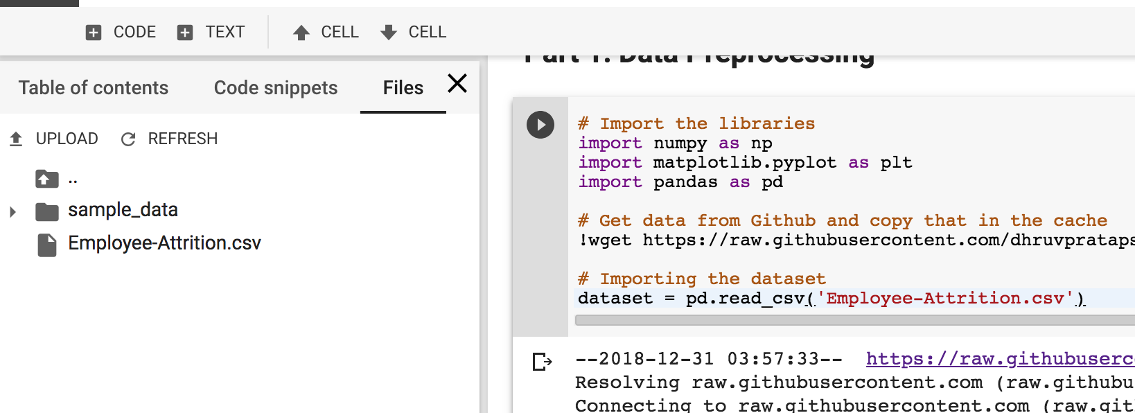
# Importing the dataset
dataset = pd.read_csv('Employee-Attrition.csv')

Intuition for Cleaning the data

1. Remove a column with same value for all the rows StandardHours Over18

2. Remove the columns with PII(Personally identifiable information) EmployeeID

3. Move y to start or the end column, to make things easier to slice (Optional)

#removing standard hours, Over18 and employeeID + attrition as first row
dataset = dataset[['Attrition',
                   'Age',
                   'BusinessTravel',
                   'DailyRate',
                   'Department',
                   'DistanceFromHome',
                   'Education',
                   'EducationField',
                   'EmployeeCount',
                   'EnvironmentSatisfaction',
                   'Gender',
                   'HourlyRate',
                   'JobInvolvement',
                   'JobLevel',
                   'JobRole',
                   'JobSatisfaction',
                   'MaritalStatus',
                   'MonthlyIncome',
                   'MonthlyRate',
                   'NumCompaniesWorked',
                   'OverTime',
                   'PercentSalaryHike',
                   'PerformanceRating',
                   'RelationshipSatisfaction',
                   'StockOptionLevel',
                   'TotalWorkingYears',
                   'TrainingTimesLastYear',
                   'WorkLifeBalance',
                   'YearsAtCompany',
                   'YearsInCurrentRole',
                   'YearsSinceLastPromotion',
                   'YearsWithCurrManager']]

Remember that in python index slicing we include the start index and exclude the end index. Use first index i.e. 0 as y (dependent variable) and 1-32 as X (independent variables)

X = dataset.iloc[:, 1:].values
y = dataset.iloc[:, 0].values

SOME TRICKS

‘print(y)’ or to see the y vector.
‘X.shape’ to see the shape of the matrix.
We use Uppercase X as it is a matrix and lowercase y as it is a vector

Encoding categorical data

As the algorithms work best with numbers.

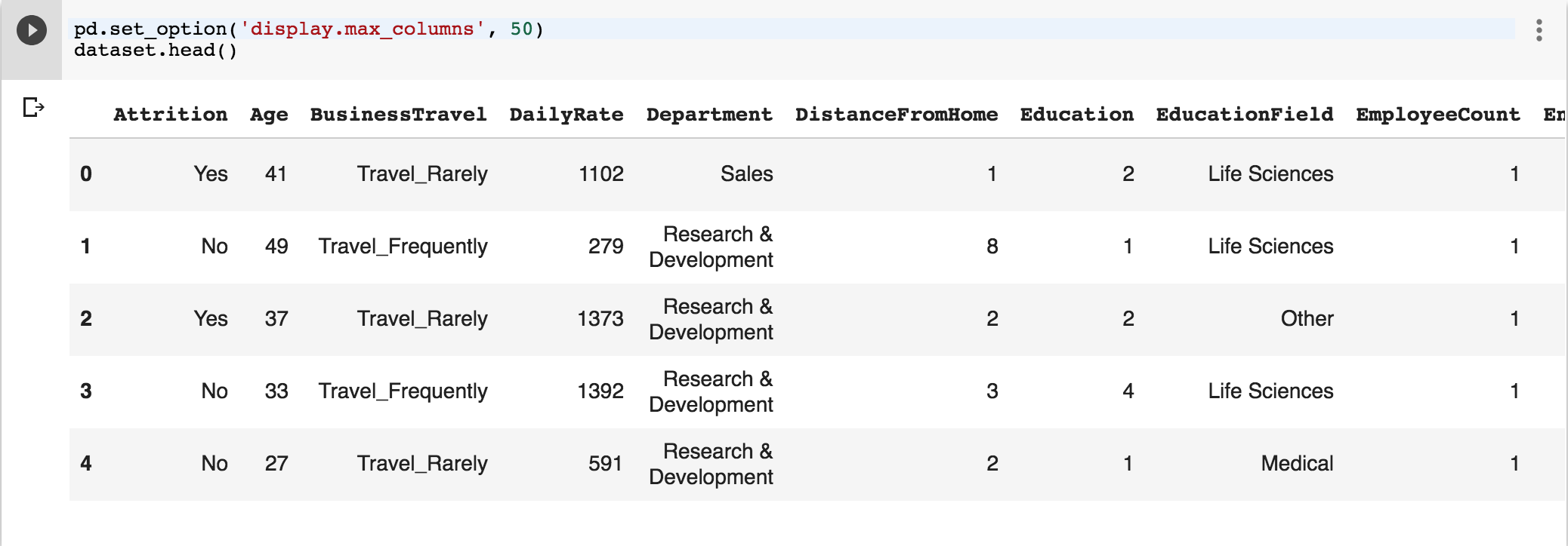
Set the display max columns to see all columns.

Columns that need to encoded:

Attrition y[0]
BusinessTravel X[1]
Department X[3]
EducationField X[6]
Gender X[9]
JobRole X[13]
MaritalStatus X[15]
OverTime X[19]

pd.set_option('display.max_columns', 50)
dataset.head()

First 5 rows look something like this… rest of the columns not in the image.

# Encoding categorical data
from sklearn.preprocessing import LabelEncoder, OneHotEncoder
labelencoder_X_1 = LabelEncoder()
X[:, 1] = labelencoder_X_1.fit_transform(X[:, 1])
labelencoder_X_2 = LabelEncoder()
X[:, 3] = labelencoder_X_2.fit_transform(X[:, 3])
labelencoder_X_3 = LabelEncoder()
X[:, 6] = labelencoder_X_3.fit_transform(X[:, 6])
labelencoder_X_4 = LabelEncoder()
X[:, 9] = labelencoder_X_4.fit_transform(X[:, 9])
labelencoder_X_5 = LabelEncoder()
X[:, 13] = labelencoder_X_5.fit_transform(X[:, 13])
labelencoder_X_6 = LabelEncoder()
X[:, 15] = labelencoder_X_6.fit_transform(X[:, 15])
labelencoder_X_7 = LabelEncoder()
X[:, 19] = labelencoder_X_7.fit_transform(X[:, 19])
labelencoder_y= LabelEncoder()
y = labelencoder_y.fit_transform(y)

#no dummy trap
onehotencoder1 = OneHotEncoder(categorical_features = [1])
X = onehotencoder1.fit_transform(X).toarray()
X = X[:,1:]
onehotencoder3 = OneHotEncoder(categorical_features = [4])
X = onehotencoder3.fit_transform(X).toarray()
X = X[:,1:]
onehotencoder6 = OneHotEncoder(categorical_features = [8])
X = onehotencoder6.fit_transform(X).toarray()
X = X[:,1:]
onehotencoder13 = OneHotEncoder(categorical_features = [19])
X = onehotencoder13.fit_transform(X).toarray()
X = X[:,1:]
onehotencoder15 = OneHotEncoder(categorical_features = [28])
X = onehotencoder15.fit_transform(X).toarray()
X = X[:,1:]

Splitt data into training and test set

# Splitting the dataset into the Training set and Test set
from sklearn.model_selection import train_test_split
X_train, X_test, y_train, y_test = train_test_split(X, y, test_size = 0.2, random_state = 0)

Feature Scaling

# Feature Scaling
from sklearn.preprocessing import StandardScaler
sc = StandardScaler()
X_train = sc.fit_transform(X_train)
X_test = sc.transform(X_test)

Part 2: Create Artificial Neural Network

# Importing the Keras libraries and packages
import keras
from keras.models import Sequential
from keras.layers import Dense
from keras.layers import Dropout
from keras.wrappers.scikit_learn import KerasClassifier
from sklearn.model_selection import cross_val_score
from sklearn.model_selection import GridSearchCV

#Parameters
dropout = 0.1
epochs = 100
batch_size = 30
optimizer = 'adam'
k = 20

def build_ann_classifier():
  # Initialising the ANN
  classifier = Sequential()

  # Adding the input layer and the first hidden layer
  classifier.add(Dense(units = 16, kernel_initializer = 'uniform', activation = 'relu', input_shape = (X.shape[1],)))

  classifier.add(Dropout(dropout))

  # Adding the output layer
  classifier.add(Dense(units = 1, kernel_initializer = 'uniform', activation = 'sigmoid'))

  # Compiling the ANN
  classifier.compile(optimizer = 'adam', loss = 'binary_crossentropy', metrics = ['accuracy'])

  return classifier

  classifier = KerasClassifier(build_fn = build_ann_classifier, batch_size = 10, epochs = epochs, verbose = 0)
  accuracies = cross_val_score(estimator = classifier, X = X_train, y = y_train, cv = 10, n_jobs = -1)
  max = accuracies.max()
  print(max)
  mean = accuracies.mean()
  variance = accuracies.std()
  print(mean)
  print(variance)

The result of this is: We got 92.3% accuracy at best.

9237288095183291
8596697045390578
030821566189208408

Tune parameters using GridSearchCV (Cross Validation)

To find the best parameters we can give grid_search some values to test and it will find the best combo.

def build_ann_classifier(optimizer):
  # Initialising the ANN
  classifier = Sequential()

  # Adding the input layer and the first hidden layer
  classifier.add(Dense(units = 16, kernel_initializer = 'uniform', activation = 'relu', input_shape = (X.shape[1],)))

  classifier.add(Dropout(dropout))

  # Adding the output layer
  classifier.add(Dense(units = 1, kernel_initializer = 'uniform', activation = 'sigmoid'))

  # Compiling the ANN
  classifier.compile(optimizer = optimizer, loss = 'binary_crossentropy', metrics = ['accuracy'])

  return classifier


classifier = KerasClassifier(build_fn = build_ann_classifier, verbose = 0)
parameters = {'batch_size': [25, 32],
              'epochs': [100],
              'optimizer': ['adam', 'rmsprop']}
grid_search = GridSearchCV(estimator = classifier,
                           param_grid = parameters,
                           scoring = 'accuracy',
                           cv = 10)
grid_search = grid_search.fit(X_train, y_train)
best_parameters = grid_search.best_params_
best_accuracy = grid_search.best_score_

Resulting best parameters:

{'batch_size': 25, 'epochs': 100, 'optimizer': 'adam'}

You can find complete python code here.

Please let me know if you have any questions or suggestions in the comments section below. Thanks.

dps.xyz